When Quantum Memories Become the Bottleneck: What Does It Take to Build a Working Quantum Network?
November 10, 2026 · David Vesterlund · Quantum networks, quantum memories, and simulation
A future quantum internet will need more than powerful quantum computers. It will need memories that can wait, nodes that can cooperate, and network architectures that put limited resources where they matter most. In my new paper in Quantum Reports, I investigate how these elements interact, and why answering the seemingly simple question, “How many quantum memories do we need?” is far more complicated than it first appears.
Read the research paper at MDPI
Memory Physics, Finite Capacity, and Topology in Heterogeneous Quantum Networks, Quantum Reports (2026), 8(4), 120. DOI: 10.3390/quantum8040120.
Imagine a network that has to wait for quantum physics
In an ordinary computer network, information travels between routers in packets. Those packets can be buffered and forwarded when a connection becomes available. A quantum network works differently. To connect distant nodes, we may need to create quantum entanglement over several shorter links, then join those links through a process called entanglement swapping.
Imagine three stations: A, B, and C. We successfully establish entanglement between A and B, but the second link, from B to C, does not succeed immediately. The first entangled state must then be preserved in a quantum memory while we try again.
This creates a difficult engineering problem. A quantum memory can preserve its state only for a limited time. Retrieving that state may fail. Each node has a finite number of memory slots, and multiple requests may compete for them. The shape of the network also determines which nodes spend the most time waiting.
A memory with an impressive coherence time is therefore not enough on its own. We need to understand how it performs alongside other memories, within a particular network topology, and under the traffic that network must support.
Four research questions and one central hypothesis about Quantum Networks
The paper begins with four questions:
- What limits the delivery of entanglement? Is the main constraint memory physics, the number of available memory slots, traffic load, or network structure?
- How does performance change across technologies and topologies? Does the same quantum memory provide the same benefit in a chain, a star, and a more richly connected network?
- Is there a simple rule for sizing memory capacity? Could one formula tell us approximately how many memory slots each node needs?
- Where should the best memories be placed? Can we build a useful network from a mix of advanced and more modest memory technologies?
My central hypothesis was that quantum-memory requirements cannot be expressed by one universal number. Memory physics, position in the network, and the demands of incoming traffic interact. Any sufficiently useful model must account for all three.
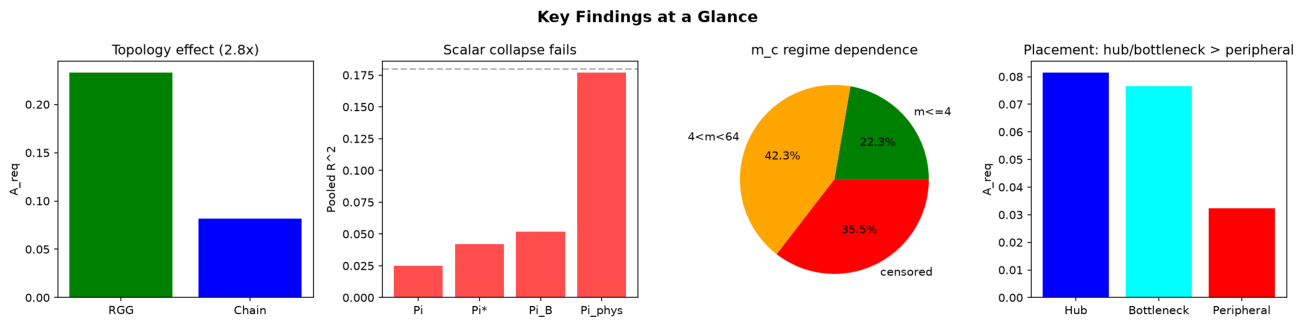
Figure 1. Overview from the openly available manuscript version. The panels illustrate differences among network topologies, the difficulty of finding a common scaling rule, variation in memory requirements, and the benefits of placing better memories at central nodes. The numerical findings apply to the simulated scenarios, not to every possible quantum network.
How I conducted the study
The study uses discrete-event simulation. Instead of attempting to reproduce every atom and photon in complete quantum-mechanical detail, the simulator tracks network events over time: a link attempts to generate entanglement, an attempt succeeds or fails, a memory slot becomes occupied, the quality of a stored quantum state degrades, and an entanglement-swapping operation is attempted.
This approach makes it possible to investigate many network designs under controlled conditions before building a physical system.
The main components of the experiments were:
- Six representative quantum-memory profiles: trapped ions, neutral atoms, electron and nuclear spins in diamond, atomic frequency comb (AFC) memories, and superconducting circuits.
- Nine network topology classes: including chains, stars, rings, lattices, trees, hierarchical structures, and random geometric graphs.
- Three network sizes: 10, 20, and 50 nodes, tested under different traffic loads and memory budgets.
- Repeated simulations: 9,360 completed runs in the main memory–topology atlas, supplemented by 8,730 runs in a confirmatory dataset.
- Additional analyses: including 840 memory-capacity threshold estimates, 5,310 heterogeneous-placement runs, and a sensitivity analysis based on 67,584 samples.
These numbers refer to separate studies with partially different experimental designs. They should not be added together and interpreted as one large set of independent observations.
The Nine Network Topologies Used in My Study
To understand how quantum memories behave in different network environments, I simulated nine network topologies. Each represents a different way of connecting quantum nodes, allowing me to study how network structure affects entanglement distribution, memory requirements, and performance.
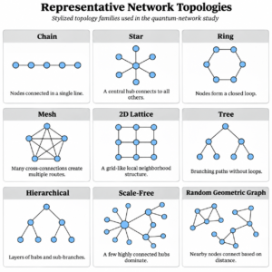
1. Chain Network
Nodes are connected in a straight line, with quantum information passing through intermediate nodes. This provides a simple baseline for studying how distance, waiting times, and memory decoherence affect performance.
2. Star Network
All nodes connect through one central hub. This helps investigate how heavily connected nodes become bottlenecks and whether placing better quantum memories at these central locations improves performance.
3. Ring Network
Nodes form a closed loop, allowing communication in two directions. This topology helps examine whether alternative routes reduce bottlenecks and improve entanglement delivery.
4. Lattice Network
Nodes are arranged in a regular grid and connected to nearby neighbors. This provides a structured environment for studying routing, memory allocation, and the effects of multiple possible paths.
5. Binary Tree Network
Nodes form a branching structure without loops. This allows me to investigate how quantum memories perform when communication must pass through specific intermediate nodes.
6. Hierarchical Network
Nodes are organized into multiple levels of interconnected groups. This helps examine how memory requirements change when communication traffic concentrates at higher-level nodes.
7. Scale-Free Network
A small number of highly connected hubs link many less-connected nodes. This topology is particularly useful for investigating where high-performance quantum memories should be placed.
8. Random Geometric Graph (RGG)
Nodes are distributed randomly in space and connect when they are sufficiently close. This models spatially constrained networks and helps reveal how physical location and connectivity influence performance.
9. Waxman Network
Connections are generated probabilistically, with nearby nodes more likely to connect than distant ones. Unlike an RGG, longer-distance links remain possible. This helps investigate how distance-dependent connectivity and network shortcuts affect quantum-memory performance.
Why Compare All Nine?
The central question is whether the same quantum-memory technology performs equally well across different network structures.
By comparing these nine topologies, I can investigate how connectivity, bottlenecks, routing alternatives, and network geometry interact with memory capacity and physical limitations.
The results suggest that there is no single optimal memory configuration for every network. Quantum-memory requirements must be evaluated together with the topology and operating conditions.
What does “performance” mean in this study?
One of the paper’s main metrics is A_req: the fraction of relevant entanglement requests completed before their deadline. Another metric, A_qual, requires the delivered entangled state to meet a minimum fidelity, meaning that it must be sufficiently close to the desired quantum state.
The two metrics answer different questions. A network may deliver a result on time while delivering entanglement of inadequate quality. That is why performance must be defined carefully before networks are compared.
Table: Which quantum-memory technologies were compared?
| Representative memory profile | Coherence time T₂ | Initial retrieval efficiency | Retrieval decay constant τᵣ |
|---|---|---|---|
| Trapped ion | 10 s | 90% | 10 s |
| Neutral atom | 0.1 s | 80% | 0.5 s |
| Diamond, electron spin | 0.044 s | 70% | 0.1 s |
| Diamond, nuclear spin | 1.3 s | 50% | 1 s |
| AFC | 0.005 s | 50% | 0.01 s |
| Superconducting circuit | 0.0001 s | 95% | 0.001 s |
Adapted from Table 2 of the published article. These are literature-informed modeling profiles, not rankings of complete commercial devices. T₂ describes the loss of quantum coherence, whereas τᵣ describes the timescale over which successful retrieval becomes less likely.
The distinction between these timescales matters. A memory may preserve an apparently useful quantum state for a relatively long time but still be difficult to read out. Another may offer high retrieval efficiency at first while rapidly losing its useful stored state.
Among the simulation’s baseline assumptions are a 0.5% chance of generating entanglement in an elementary link attempt, 1 millisecond between attempts, a 98% success probability for an entanglement-swapping attempt, and a one-second request deadline. These are experimental assumptions, not universal specifications for quantum-network hardware.
Finding 1: More quantum memories help, but with diminishing returns
The first practical question is straightforward: What happens when each node receives additional memory slots?
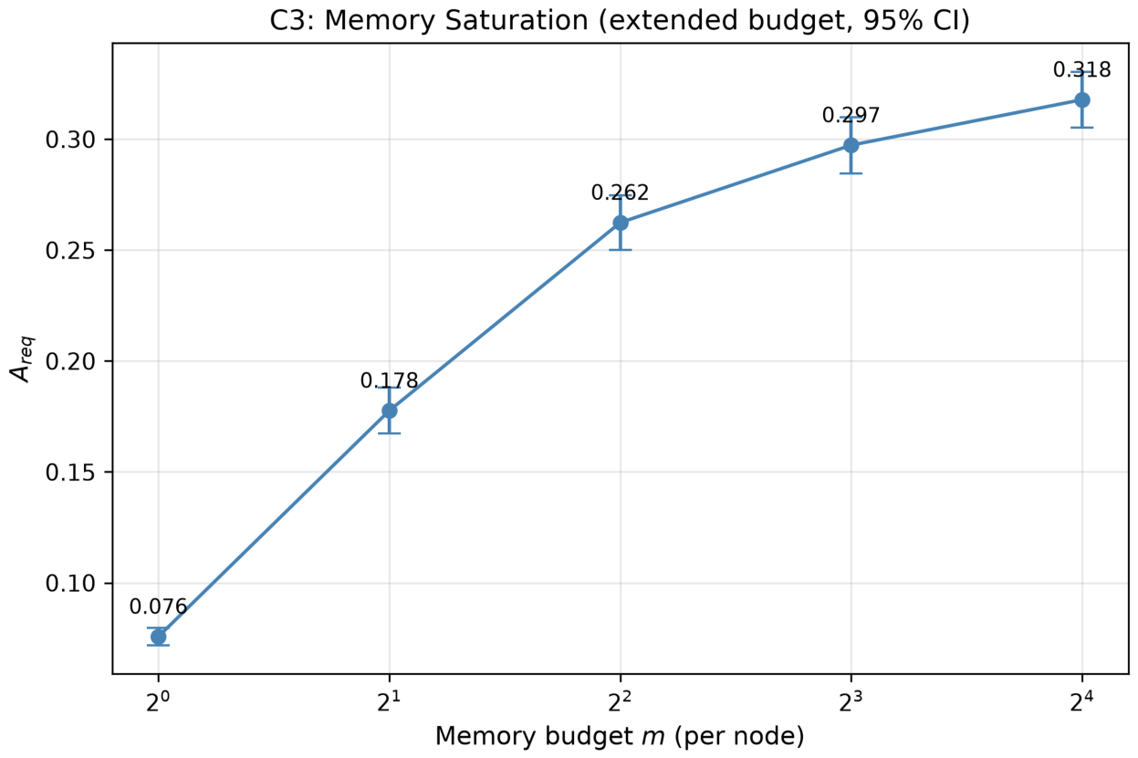
Figure 2. Average request completion fraction, A_req, as the number of memory slots per node increases from 1 to 16. Error bars show 95% confidence intervals. This is Figure 2 from the manuscript version.
When the budget increases from one to two memory slots, average on-time delivery rises from 7.6% to 17.8%. With four slots, it reaches 26.2%; with eight, 29.7%; and with sixteen, 31.8%.
The result shows clear diminishing marginal returns. The first extra memory slots make a substantial difference. Further additions help, but by progressively smaller amounts. The curve does not, however, establish a fundamental upper limit: performance could continue to improve with more than sixteen slots.
There is an important difference between watching a curve begin to flatten and demonstrating that the system has reached its ultimate capacity.
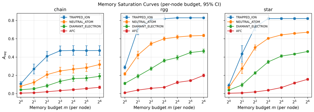
Figure 3. Each panel represents a network topology, and each colored curve represents a memory profile. The horizontal axis shows memory slots per node, from 1 to 64; the vertical axis shows the request completion fraction.
Consider the trapped-ion curve first. Under the tested parameters, it approaches a region relatively quickly where additional slots provide little benefit. By contrast, the AFC curve is still rising at the largest tested memory budget.
This does not establish that AFC technology is generally inferior to trapped-ion memories. AFC systems may offer important advantages for optical storage and multimode operation, which these simplified profiles do not fully capture. The result tells us that the particular modeled memory profiles respond differently to network demands.
The plots also show that network geometry matters. In the confirmatory experiments, random geometric graphs achieved a mean A_req of 0.233, compared with 0.082 for chains, a difference of approximately 2.8 times. But this cannot be attributed to topology alone: path lengths and the total memory available in the network may also differ.
Finding 2: There is no single memory-slot count that works everywhere
To study capacity requirements, I defined a practical threshold called m_c. It is the smallest tested per-node memory budget that achieves 95% of the best performance actually observed across the tested budgets of 1, 2, 4, 8, 16, 32, and 64 slots.
The words actually observed are essential. If performance is still improving at 64 slots, the experiment has not yet located the network’s true long-run plateau.
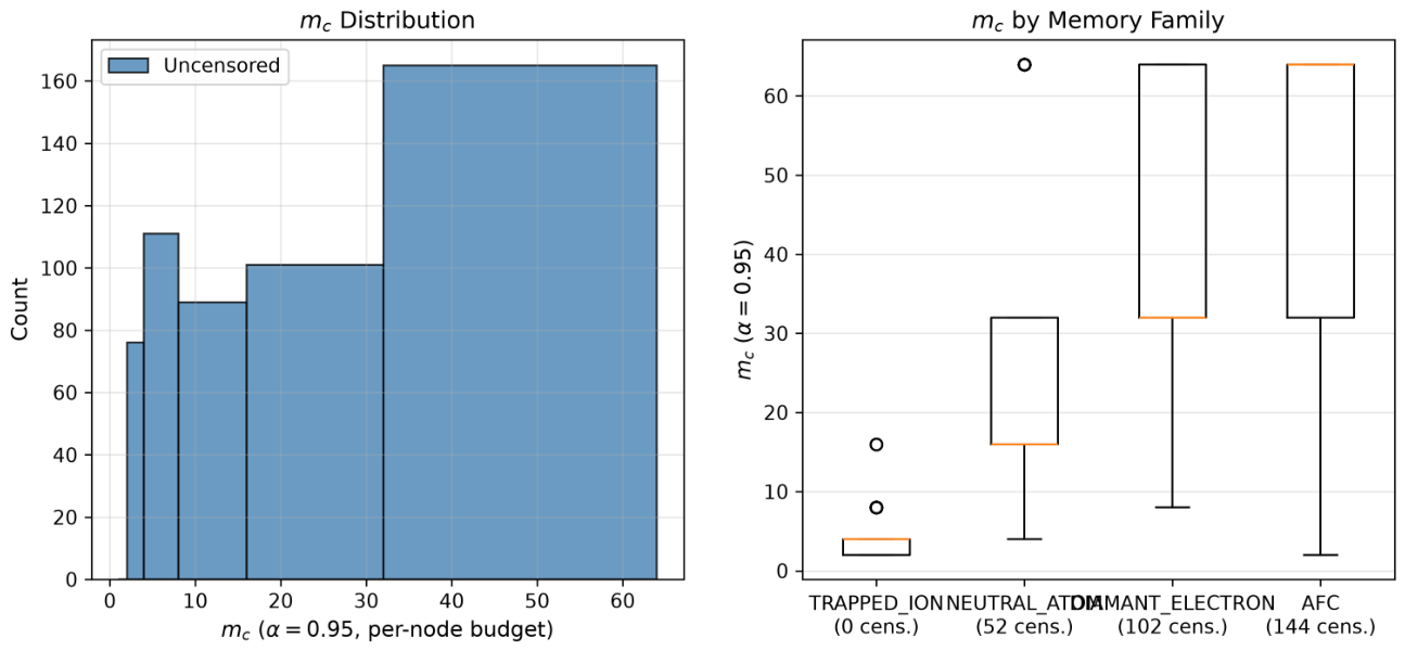
Figure 4. The left-hand panel shows the distribution of capacity thresholds across simulated scenarios; the right-hand panel compares memory profiles. A threshold recorded at 64 is a boundary case of the tested grid, not proof that 64 slots is the ultimate optimal capacity.
| Memory profile | Median m_c | Scenarios first reaching the criterion at 64 slots |
|---|---|---|
| Trapped ion | 4 | 0 of 210 |
| Neutral atom | 16 | 52 of 210 |
| Diamond, electron spin | 32 | 102 of 210 |
| AFC | 64, upper test boundary | 144 of 210 |
Adapted from Table 5 of the published article. All values refer to 95% of the best observed result on a finite memory-budget grid.
Across 840 evaluated scenarios, 22.3% met the criterion with no more than four slots, while 35.5% first met it at the upper test boundary of 64 slots.
With such wide variation, it is hard to give useful advice such as “a quantum network needs eight memories per node.” The appropriate number depends on the hardware profile, traffic pattern, and position of the nodes.
Finding 3: An elegant formula is not enough, at least not yet
Mathematicians and engineers often look for scaling laws: compact relationships that predict the behavior of many different systems. If quantum-network performance could be reduced to a single dimensionless variable, network sizing would become much easier.
I tested four candidate reductions. They combined information about traffic, available memory, link-generation probabilities, route lengths, congestion at central nodes, and memory physics in different ways.
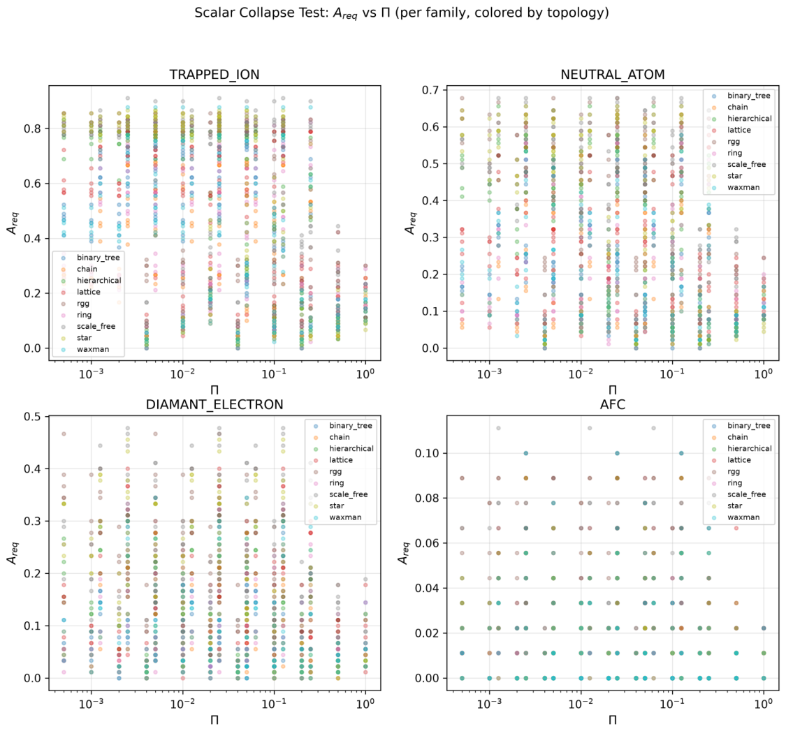
Figure 5. Each point represents a simulated scenario. If the proposed variable summarized network behavior well, the points would cluster around a common relationship. Instead, substantial differences remain, even within the same memory profile.
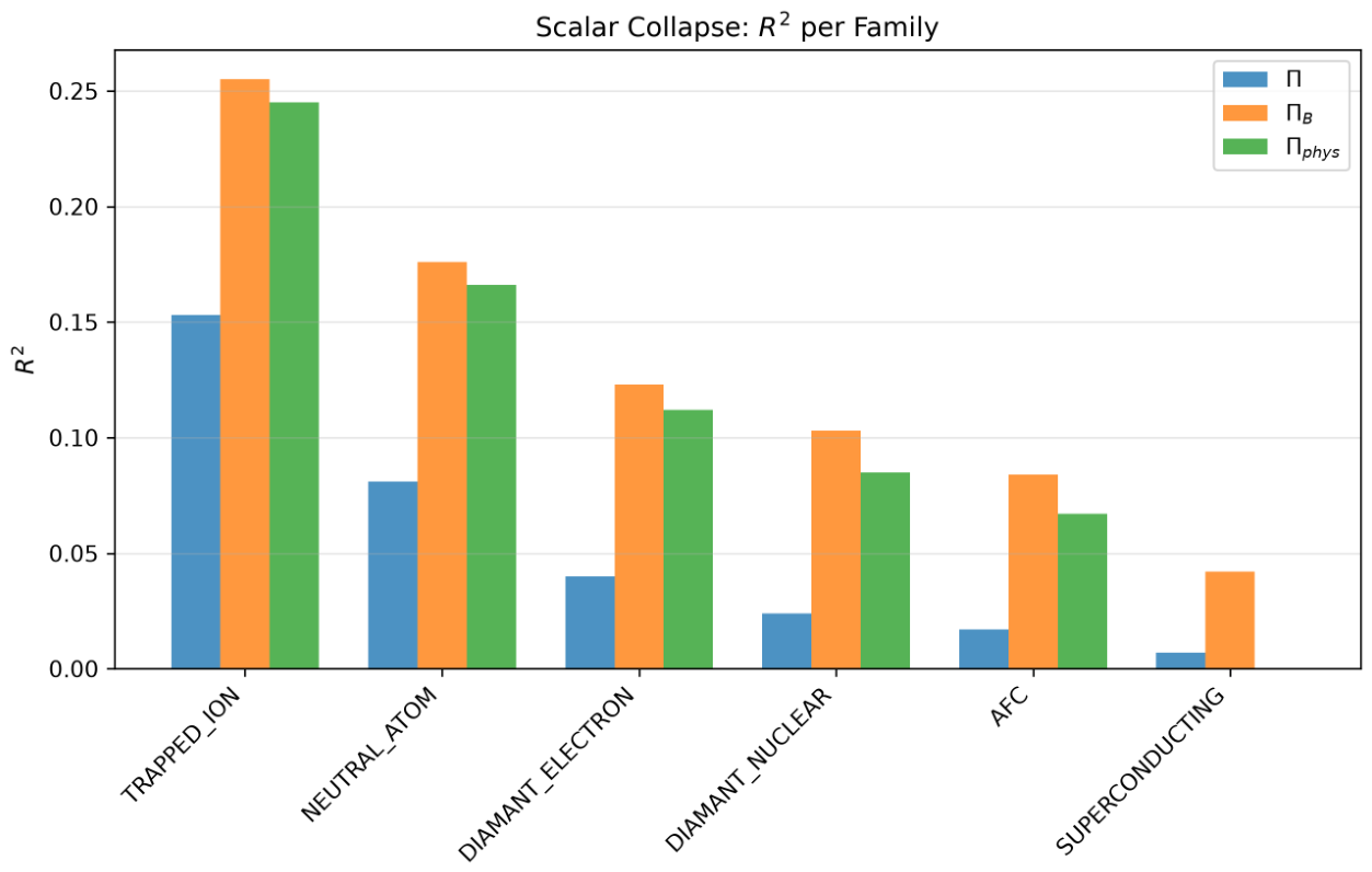
Figure 6. The bars show R², a statistical measure of how well a fitted model explains variation. A value of 1 means a perfect fit, while 0 means no improvement over a constant baseline. None of the tested scalar variables provides a strong explanation across all memory profiles.
| Tested description | R², linear fit in log space | R², quadratic fit in log space |
|---|---|---|
| Traffic relative to memory capacity (Π) | 0.025 | 0.029 |
| Same quantity adjusted for path length (Π*) | 0.042 | 0.045 |
| Bottleneck load (Π_B) | 0.052 | 0.058 |
| Physics-adjusted quantity (Π_phys) | 0.177 | 0.379 |
Adapted from Table 8 of the published article, using the pooled results.
The best linear model explained only 17.7% of the variation. Allowing a nonlinear, quadratic relationship increased the best fit to 37.9%, but much of the apparent improvement reflected differences between memory profiles, rather than one common law that worked within each profile.
The conclusion is specific but important: these four candidate reductions are not universal memory-sizing rules in the tested scenarios. The study does not prove that a more successful general law is mathematically impossible.
A more physical way to understand the differences
A more physically motivated idea is to ask how many successful link-generation attempts we expect during the period in which a stored quantum state can still be retrieved. This leads to a dimensionless quantity:
χᵣ = τᵣ × p_gen / t_attempt.
Here τᵣ is the retrieval decay time, p_gen is the probability that a link-generation attempt succeeds, and t_attempt is the time between attempts.
When χᵣ is small, the opportunity for different links to succeed while a stored state remains retrievable is limited. When χᵣ is large, bottlenecks are more likely to involve queueing, offered traffic, and competition for available memory slots.
This distinction helps us interpret the simulated operating regimes. It does not yet provide a validated formula for the number of memory slots required by a real-world quantum network.
Finding 4: Where the best memories are placed can matter as much as how many there are
A future quantum network is unlikely to consist of identical nodes. Some sites may have expensive, high-performance memories, while others use cheaper or technically different devices.
I therefore compared strategies for deciding where higher-quality memories should be installed.
A hub is a node connected directly to many neighbors. A bottleneck node lies on many of the network’s shortest paths. A peripheral node sits farther from the principal traffic routes.
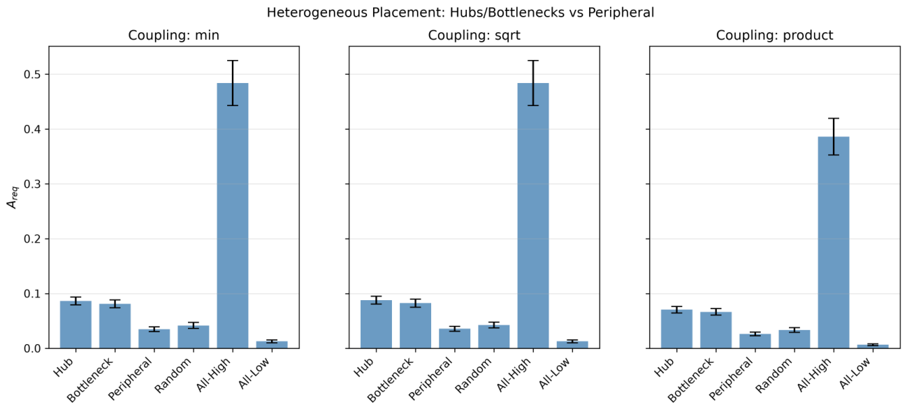
Figure 7. On average, placing better memories at hubs and bottlenecks improves performance more than putting those same resources at peripheral nodes. The much higher “All-High” bar represents the more costly alternative in which every node receives the better memory profile.
| Placement of higher-quality memories | Mean A_req |
|---|---|
| Central hubs | 0.0815 |
| Traffic bottlenecks | 0.0766 |
| Peripheral nodes | 0.0323 |
Summary of results in Section 9 of the published paper; these values are not copied from a separate published table.
The finding points to a practical principle: when advanced memories are expensive, we should first identify which nodes influence the largest number of paths and requests.
There are two important caveats. First, hub and bottleneck strategies had very similar practical effects even where a statistical difference could be detected. Second, the ranking varied by topology; in some networks, other placements performed better.
Assumptions about the interface between two different memory platforms also substantially changed the absolute performance values. Optimizing placement on an elegant-looking network graph is therefore not enough. The interfaces between hardware technologies must be modeled explicitly.
Finding 5: Which properties tell us the most about network performance?
As a complementary analysis, I used a Random Forest machine-learning model to predict network performance from the parameters varied in the simulations.
The model was trained and evaluated separately for three topology classes. I then tested how much its predictions deteriorated when one input parameter at a time was randomly shuffled, an approach known as permutation importance.
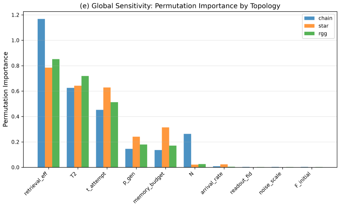
Figure 8. Across the tested topologies, the parameter with the greatest influence on the model’s predictions was retrieval efficiency. Other influential variables included the coherence time T₂ and the interval between link-generation attempts.
| Evaluation group | R² on held-out test data |
|---|---|
| Chain networks | 0.944 |
| Star networks | 0.972 |
| Random geometric graphs | 0.974 |
| All three pooled together | 0.423 |
Adapted from Table 10 of the published article. A high R² within one topology means the model captures patterns in that particular dataset; it does not establish generalization to unseen topologies or physical networks.
Why does the result deteriorate so much when the datasets are pooled? One likely reason is that network structure matters, while the pooled model was not explicitly given topology as an input feature. This is another illustration of the paper’s central theme: a relationship that works within one family of networks may fail to explain another.
There is also a statistical trap. In the selected memory profiles, T₂ and the retrieval decay constant can vary together. A Random Forest model may therefore use one as an indirect proxy for the other. Predictive importance is not proof of physical causation.
What these results mean, and what they do not prove
The study suggests three practical lessons for the design of future quantum networks.
First: memory capacity should be sized for how a network is actually used. A fixed number of memory slots per node is a weak general design rule.
Second: network geometry and traffic flows affect the value of advanced hardware. Placing the right memory technology in the wrong location may offer less benefit than a more carefully targeted allocation of resources.
Third: quantum memories cannot be judged solely by how long they preserve coherence. It also matters how quickly and reliably the state can be retrieved, and how the memory interacts with the rest of the network.
It is equally important to distinguish patterns found in simulations from experimentally verified physical results. The memory profiles are simplified parameter bundles. The model does not include every possible protocol or technology, such as comprehensive entanglement purification and multiplexing. Some topology comparisons are influenced by unequal total memory budgets, and the highest traffic loads were simulated over relatively short observation periods.
Selected conclusions were also tested using harmonized implementations on the SeQUeNCe and SimQN event frameworks. Those checks supported certain relative rankings, but they are not equivalent to independent replications using each framework’s full native protocols.
This paper is therefore not a blueprint for a finished quantum internet tomorrow. It is a step toward better capacity-planning methods, experimental comparisons, and testable engineering hypotheses.
Next steps: From simulated network physics to real design decisions
For me, one of the most interesting implications is that optimizing individual components in isolation will not be enough.
The next research steps are to test these findings against more independent network models, use more detailed and experimentally measured hardware profiles, hold the total available memory constant when comparing topologies, and describe interfaces between different memory technologies more faithfully. In the longer term, we also need physical experiments with real hardware and realistic traffic.
The goal is not merely to ask how good a quantum memory is in a laboratory. It is to answer a more useful question:
How much will this particular memory improve a real quantum network, in this particular location, under these particular conditions?
That is where memory physics, network mathematics, and engineering begin to meet.
Read the original paper
David Vesterlund (2026). Memory Physics, Finite Capacity, and Topology in Heterogeneous Quantum Networks. Quantum Reports, 8(4), 120. DOI: 10.3390/quantum8040120.
Read the open-access article at MDPI.
Figures 1–8 above are linked from the openly available preprint version of the same study, with attribution under CC BY 4.0. The published article at MDPI should be used for formal citation.